Welcome to the second project of the Machine Learning Engineer Nanodegree! In this notebook, some template code has already been provided for you, and it will be your job to implement the additional functionality necessary to successfully complete this project. Sections that begin with 'Implementation' in the header indicate that the following block of code will require additional functionality which you must provide. Instructions will be provided for each section and the specifics of the implementation are marked in the code block with a 'TODO' statement. Please be sure to read the instructions carefully!
In addition to implementing code, there will be questions that you must answer which relate to the project and your implementation. Each section where you will answer a question is preceded by a 'Question X' header. Carefully read each question and provide thorough answers in the following text boxes that begin with 'Answer:'. Your project submission will be evaluated based on your answers to each of the questions and the implementation you provide.
Note: Code and Markdown cells can be executed using the Shift + Enter keyboard shortcut. In addition, Markdown cells can be edited by typically double-clicking the cell to enter edit mode.
# reset the ipython
%reset
Question 1 - Classification vs. Regression
Your goal for this project is to identify students who might need early intervention before they fail to graduate. Which type of supervised learning problem is this, classification or regression? Why?
Answer:
This type of supervised learning a classification problem. Because the target output is categorical data as
YesorNo(binary value) report whether a student pass the final exam.
Exploring the Data
Run the code cell below to load necessary Python libraries and load the student data. Note that the last column from this dataset, 'passed', will be our target label (whether the student graduated or didn't graduate). All other columns are features about each student.
# Import libraries
import numpy as np
import pandas as pd
from time import time
from sklearn.metrics import f1_score

# Read student data
student_data = pd.read_csv("student-data.csv")
print "Student data read successfully!"
# Import libraries
from sklearn import metrics
import matplotlib.pyplot as plt

%matplotlib inline
from IPython.display import display

# - store inline rc to recover defaults later
# - matplotlib defaults: mpl.rcParams.update(mpl.rcParamsDefault)
import matplotlib as mpl
inline_rc = dict(mpl.rcParams)
# - recover defaults from stored inline rc
mpl.rcParams.update(inline_rc)
print "Import libraries successfully! (^^)v"
Implementation: Data Exploration
Let's begin by investigating the dataset to determine how many students we have information on, and learn about the graduation rate among these students. In the code cell below, you will need to compute the following:
- The total number of students,
n_students. - The total number of features for each student,
n_features. - The number of those students who passed,
n_passed. - The number of those students who failed,
n_failed. - The graduation rate of the class,
grad_rate, in percent (%).
# TODO: Calculate number of students
n_students = len(student_data)
# TODO: Calculate number of features
# Total number of column - 1, which is the target label
n_features = len(student_data.columns) - 1
# TODO: Calculate passing students
n_passed = student_data.passed.value_counts()['yes']
# TODO: Calculate failing students
n_failed = student_data.passed.value_counts()['no']
# TODO: Calculate graduation rate
grad_rate = float(n_passed) / n_students * 100

# Print the results
print "Total number of students: {}".format(n_students)
print "Number of features: {}".format(n_features)
print "Number of students who passed: {}".format(n_passed)
print "Number of students who failed: {}".format(n_failed)
print "Graduation rate of the class: {:.2f}%".format(grad_rate)
# do: print the F1 score
print "\nF1 score for all 'yes' on students: {:.4f}".format(
    f1_score(y_true = ['yes'] * n_passed + ['no'] * n_failed,
             y_pred = ['yes'] * n_students, pos_label = 'yes', average = 'binary'))
Preparing the Data
In this section, we will prepare the data for modeling, training and testing.
Identify feature and target columns
It is often the case that the data you obtain contains non-numeric features. This can be a problem, as most machine learning algorithms expect numeric data to perform computations with.
Run the code cell below to separate the student data into feature and target columns to see if any features are non-numeric.
# Extract feature columns
feature_cols = list(student_data.columns[:-1])

# Extract target column 'passed'
target_col = student_data.columns[-1]

# Show the list of columns
print "Feature columns:\n{}".format(feature_cols)
print "\nTarget column: {}".format(target_col)

# Separate the data into feature data and target data (X_all and y_all, respectively)
X_all = student_data[feature_cols]
y_all = student_data[target_col]

# Show the feature information by printing the first five rows
print "\nFeature values:"
display(X_all.head())
Preprocess Feature Columns
As you can see, there are several non-numeric columns that need to be converted! Many of them are simply yes/no, e.g. internet. These can be reasonably converted into 1/0 (binary) values.
Other columns, like Mjob and Fjob, have more than two values, and are known as categorical variables. The recommended way to handle such a column is to create as many columns as possible values (e.g. Fjob_teacher, Fjob_other, Fjob_services, etc.), and assign a 1 to one of them and 0 to all others.
These generated columns are sometimes called dummy variables, and we will use the pandas.get_dummies() function to perform this transformation. Run the code cell below to perform the preprocessing routine discussed in this section.
def preprocess_features(X):
    ''' Preprocesses the student data and converts non-numeric binary variables into
        binary (0/1) variables. Converts categorical variables into dummy variables. '''

    # Initialize new output DataFrame
    output = pd.DataFrame(index = X.index)

    # Investigate each feature column for the data
    for col, col_data in X.iteritems():

        # If data type is non-numeric, replace all yes/no values with 1/0
        if col_data.dtype == object:
            col_data = col_data.replace(['yes', 'no'], [1, 0])

        # If data type is categorical, convert to dummy variables
        if col_data.dtype == object:
            # Example: 'school' => 'school_GP' and 'school_MS'
            col_data = pd.get_dummies(col_data, prefix = col)

        # Collect the revised columns
        output = output.join(col_data)

    return output

X_all = preprocess_features(X_all)
print "Processed feature columns ({} total features):\n{}".format(len(X_all.columns), list(X_all.columns))
Implementation: Training and Testing Data Split
So far, we have converted all categorical features into numeric values. For the next step, we split the data (both features and corresponding labels) into training and test sets. In the following code cell below, you will need to implement the following:
- Randomly shuffle and split the data (
X_all,y_all) into training and testing subsets.- Use 300 training points (approximately 75%) and 95 testing points (approximately 25%).
- Set a
random_statefor the function(s) you use, if provided. - Store the results in
X_train,X_test,y_train, andy_test.
# TODO: Import any additional functionality you may need here
from sklearn.cross_validation import train_test_split

# TODO: Set the number of training points
# Use 300 training points (approximately 75%) and 95 testing points (approximately 25%).
num_train = 300

# Set the number of testing points
num_test = X_all.shape[0] - num_train

# TODO: Shuffle and split the dataset into the number of training and testing points above
X_train, X_test, y_train, y_test = train_test_split(X_all, y_all, test_size = num_test, random_state = 42)

# Show the results of the split
print "Training set has {} samples.".format(X_train.shape[0])
print "Testing set has {} samples.".format(X_test.shape[0])
# Show the grad rates
print 'Training set grad rate: {}'.format(np.true_divide(sum(y_train == 'yes'), len(y_train)))
print 'Test set grad rate: {}'.format(np.true_divide(sum(y_test == 'yes'), len(y_test)))
Training and Evaluating Models
In this section, you will choose 3 supervised learning models that are appropriate for this problem and available in scikit-learn. You will first discuss the reasoning behind choosing these three models by considering what you know about the data and each model's strengths and weaknesses. You will then fit the model to varying sizes of training data (100 data points, 200 data points, and 300 data points) and measure the F1 score. You will need to produce three tables (one for each model) that shows the training set size, training time, prediction time, F1 score on the training set, and F1 score on the testing set.
The following supervised learning models are currently available in scikit-learn that you may choose from:
- Gaussian Naive Bayes (GaussianNB)
- Decision Trees
- Ensemble Methods (Bagging, AdaBoost, Random Forest, Gradient Boosting)
- K-Nearest Neighbors (KNeighbors)
- Stochastic Gradient Descent (SGDC)
- Support Vector Machines (SVM)
- Logistic Regression
Question 2 - Model Application
List three supervised learning models that are appropriate for this problem. For each model chosen
- Describe one real-world application in industry where the model can be applied. (You may need to do a small bit of research for this — give references!)
- What are the strengths of the model; when does it perform well?
- What are the weaknesses of the model; when does it perform poorly?
- What makes this model a good candidate for the problem, given what you know about the data?
Answer:
Consider the 3 point of reasons:
- Large number of features: Model should be able suitable for high dimension dataset
- Preferably few dataset to be used: Model that requires large dataset to train will not be preferred.
- Computational power to run the model should not be excessive
I do research on 3 models, and plus 1 more for comparing:
- Decision Tree Classifier
- Support Vector Machine (SVM)
- K-Nearest Neighbors
- Naive Base Classifer.
1. Decision Tree
1.1 General Application
- Sort of common applications of classification on text classification, Member, behavior, safety, and so on.
1.2 Strength
- Simple to visualise, understand and interpret
- Requires little data preparation, and effective in the number of data required to make prediction
- Able to handle both numerical and categorical data
- Performs well with large datasets, and the well reliability
- Possible to validate a model using statistical tests.
1.3 Weakness
- Tendency to over-fit. Minium Sample split need to be adjust to minimise. Trees can be unstable, and small variation in dataset can change the outcome of the decision tree significantly. An ensemble,which use an algorithm to compute a final prediction base on individual weighted ones is used to reduce this problem.
- The problem of learning an optimal decision tree is known to be NP-complete under several aspects of optimality and even for simple concepts; Decision-tree learners can create over-complex trees that do not generalise well from the training data; There are concepts that are hard to learn because decision trees do not express them easily, such as XOR, parity or multiplexer problems. In such cases, the decision tree becomes prohibitively large.
1.4 Reason for candidate
- It is easy to explain to the board members how the classifier algorithm works. Although features are large, not all will be used after the pruning process which can reduce the noise from the large number of features in the dataset. It also does not requires excessive dataset or computational power compared to other models.
2. Support Vector Machine (SVC)
2.1 General Application
- SVMs are helpful in text and hypertext categorization, classification of images and in medical science to classify proteins of the compounds classified correctly, and also useful in medical science to classify proteins with up to 90% of the compounds classified correctly; Hand-written characters can be recognized using SVM.
2.2 Strength
- Effective in high dimensional space and memory efficient.
- Kernel function also allow domain knowledge to be added if we know the distribution of the dataset.
- The kernel implicitly contains a non-linear transformation, no assumptions about the functional form of the transformation, which makes data linearly separable, is necessary.
- The transformation occurs implicitly on a robust theoretical basis and human expertise judgement beforehand is not needed; SVMs provide a good out-of-sample generalization, if the parameters C and r (in the case of a Gaussian kernel) are appropriately chosen.
- By choosing an appropriate generalization grade, SVMs can be robust, even when the training sample has some bias.
2.3 Weakness
- SVM gives poor result if number of features are larger than number of data.
- More difficult for board management to understand the detailed algorithm that is use derive this classifer.
- Lack of transparency of results.
2.4 Reason for candidate
- As it is suitable for high dimensional dataset and is a binary classfier, SVM fits the requirement of the dataset.
3. K-Nearest Neighbors (KNeighbors)
3.1 General Application
- Gennerally used for classification and regression problems, a successful application is the fault detection in industrial processes.
3.2 Strength
- Very robust supervised learning, when have noisy training data and work very well need to training with a large database.
- Easy to understand, however works incredibly well.
3.3 Weakness
- High computating cost for training, because need to compute distance of each query instance to all training samples, and when the number of features grows, the data grows exponentially.
3.4 Reason for candidate
- K-Nearest Neighbors may do well in generalizing data and membership and if the evaluation shows close into an existing group, the K-Nearest Neighbors can easily clarify it based on distance from other members of its class.
4. Gaussian Naive Bayes (GaussianNB)
4.1 General Application
- Gaussian Naive Bayes is used by tech companies, such as marking an detection of spam emaila, and other field like medical field to optimise treatment condition.
4.2 Strength
- Estimate each features as 1-dimensional which help minimise problems that arising from the curse of dimenionsality
- Fast computation speed.
4.3 Weakness
- Needs to be fed enough data to make reasonable accurate prediction
- Bad estimator and its output probability is not as useful(not applicable for this project requirement)
4.4 Reason for candidate
- As the dataset used contain a large number of features, Gaussian Naive Bayes would be able to show result that minimise problems from the curse of dimensionality. It is also fast to compute. The only challlenge is determining the amount of dataset needed to make accurate prediction.
Setup
Run the code cell below to initialize three helper functions which you can use for training and testing the three supervised learning models you've chosen above. The functions are as follows:
train_classifier- takes as input a classifier and training data and fits the classifier to the data.predict_labels- takes as input a fit classifier, features, and a target labeling and makes predictions using the F1 score.train_predict- takes as input a classifier, and the training and testing data, and performstrain_clasifierandpredict_labels.- This function will report the F1 score for both the training and testing data separately.
def train_classifier(clf, X_train, y_train):
    ''' Fits a classifier to the training data. '''

    # Start the clock, train the classifier, then stop the clock
    start = time()
    clf.fit(X_train, y_train)
    end = time()

    # Print the results
    print "Trained model in {:.4f} seconds".format(end - start)


def predict_labels(clf, features, target):
    ''' Makes predictions using a fit classifier based on F1 score. '''

    # Start the clock, make predictions, then stop the clock
    start = time()
    y_pred = clf.predict(features)
    end = time()

    # Print and return results
    print "Made predictions in {:.4f} seconds.".format(end - start)
    return f1_score(target.values, y_pred, pos_label='yes')


def train_predict(clf, X_train, y_train, X_test, y_test):
    ''' Train and predict using a classifer based on F1 score. '''

    # Indicate the classifier and the training set size
    print "Training a {} using a training set size of {}. . .".format(clf.__class__.__name__, len(X_train))

    # Train the classifier
    train_classifier(clf, X_train, y_train)

    # Print the results of prediction for both training and testing
    print "F1 score for training set: {:.4f}.".format(predict_labels(clf, X_train, y_train))
    print "F1 score for test set: {:.4f}.".format(predict_labels(clf, X_test, y_test))
Implementation: Model Performance Metrics
With the predefined functions above, you will now import the three supervised learning models of your choice and run the train_predict function for each one. Remember that you will need to train and predict on each classifier for three different training set sizes: 100, 200, and 300. Hence, you should expect to have 9 different outputs below — 3 for each model using the varying training set sizes. In the following code cell, you will need to implement the following:
- Import the three supervised learning models you've discussed in the previous section.
- Initialize the three models and store them in
clf_A,clf_B, andclf_C.- Use a
random_statefor each model you use, if provided. - Note: Use the default settings for each model — you will tune one specific model in a later section.
- Use a
- Create the different training set sizes to be used to train each model.
- Do not reshuffle and resplit the data! The new training points should be drawn from
X_trainandy_train.
- Do not reshuffle and resplit the data! The new training points should be drawn from
- Fit each model with each training set size and make predictions on the test set (9 in total).
Note: Three tables are provided after the following code cell which can be used to store your results.
# TODO: Import the three supervised learning models from sklearn
from sklearn import tree
from sklearn import svm
from sklearn.neighbors import KNeighborsClassifier
from sklearn.naive_bayes import GaussianNB
from sklearn import linear_model

# TODO: Initialize the three models
# Set 3-model: Decision Tree; SVC; KNeighborsClassifier; GaussianNB [delete: linear_model.LogisticRegression()]
# Set the training size: 100, 200, 300

# TODO: Execute the 'train_predict' function for each classifier and each training set size
# The 3-size loop with the 4-model loop:
classifiers = [tree.DecisionTreeClassifier(random_state=42), svm.SVC(random_state=42),
               KNeighborsClassifier(), GaussianNB()]
train_sizes = [100, 200, 300]

for clf in classifiers:
    print "\n[Result] model classifier: {} \n".format(clf.__class__.__name__)
    for n in train_sizes:
        train_predict(clf, X_train[:n], y_train[:n], X_test, y_test)
        print "---"
# helper function to train all the models and training set sizes
def train_predict_helper(clf, X_train, y_train, X_test, y_test):

    # fit training data
    start = time()
    clf.fit(X_train, y_train)
    end = time()

    # get training time and score
    time_train = end - start
    y_pred = clf.predict(X_train)
    f1_train = f1_score(y_train, y_pred, pos_label = 'yes', average = 'binary')

    # predict the test data
    start = time()
    y_pred = clf.predict(X_test)
    end = time()

    # get training time and score
    time_test = end - start
    f1_test = f1_score(y_test, y_pred, pos_label = 'yes', average = 'binary')

    return time_train, time_test, f1_train, f1_test

# Loop for tabular
clf_scores = pd.DataFrame(columns = ['Training Set Size',
                                     'Training Time',
                                     'Prediction Time (test)',
                                     'F1 Score (train)',
                                     'F1 Score (test)'])
for clf in classifiers:
    # placeholders for our results
    time_train = []; time_test = []; f1_train = []; f1_test = []

    # output the name of each classifier trained
    print "\nClassifer - {}".format(clf.__class__.__name__)

    for n in train_sizes:
        # numtrain.append(n)
        # get results for the classifier with training size n
        out = train_predict_helper(clf, X_train[:n], y_train[:n], X_test, y_test)
        # append new results
        time_train.append(out[0])
        time_test.append(out[1])
        f1_train.append(out[2])
        f1_test.append(out[3])

    results = {'Training Set Size':train_sizes,
               'Training Time': time_train,
               'Prediction Time (test)': time_test,
               'F1 Score (train)': f1_train,
               'F1 Score (test)': f1_test}

    df_results = pd.DataFrame(data = results,
                              columns = ['Training Set Size',
                                         'Training Time',
                                         'Prediction Time (test)',
                                         'F1 Score (train)',
                                         'F1 Score (test)'])

    # Tabular the results of models trained
    display(df_results)
Choosing the Best Model
In this final section, you will choose from the three supervised learning models the best model to use on the student data. You will then perform a grid search optimization for the model over the entire training set (X_train and y_train) by tuning at least one parameter to improve upon the untuned model's F1 score.
Question 3 - Choosing the Best Model
Based on the experiments you performed earlier, in one to two paragraphs, explain to the board of supervisors what single model you chose as the best model. Which model is generally the most appropriate based on the available data, limited resources, cost, and performance?
Answer:
Based on the result tables, we see that prediction time for all three models are considerably short. Therefore, my selection mainly based on the training size required and F1 score for test data.
Since we would prefer training size that small and avoding bias, the model that can make accurate prediction with the smallest training size is preferred. On these consideration, I prefer to chose SVM as the best model given its F1 score of 0.877698 with training size of 100. It also perform better than other model at the respective training sizes.
Question 4 - Model in Layman's Terms
In one to two paragraphs, explain to the board of directors in layman's terms how the final model chosen is supposed to work. Be sure that you are describing the major qualities of the model, such as how the model is trained and how the model makes a prediction. Avoid using advanced mathematical or technical jargon, such as describing equations or discussing the algorithm implementation.
Answer:
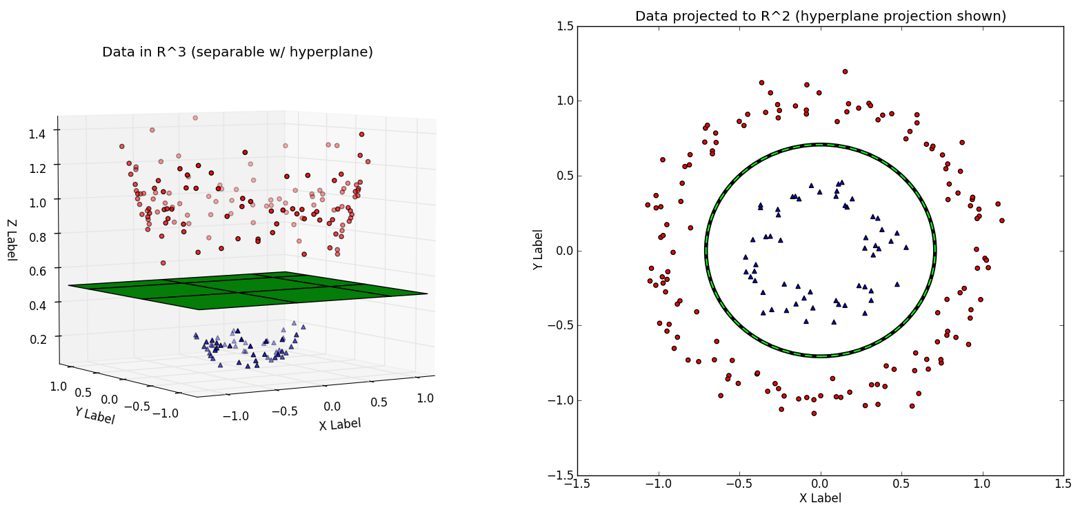
By given a new example, the naive Bayes model will first calculate the probability that this student will pass based on his or her features, $P(y_i = 1 ~|~ x_i)$, and the probability that he or she will fail, $P(y_i = 0 ~|~ x_i)$. Then the model will predict the result who has a higher probability. Support Vector Machine (SVM) is a classifier that creat a boundary between 2 classes in a dataset while maximising the distance between the boundary and class on each side. The given data points each belong to one of two classes, and the goal is to decide which class a new data point will be in. In this case, the two classes in the dataset are students that needs intervention and those that do not need.
By the case using SVM, a data point is viewed as a N-dimensional vector (a list of N-numbers), and our target is to know whether such points with a (N-1)-dimensional hyperplane can be separated. So, we chose the nearest distance data to each side is maximized. The SVM will aim to maximise this distance on both side so as not to create a bias in the data. The parameter of SVM can be adjust so that we can strike a balance between making the least classifier error and maximising the margin. Making zero classifier error is not always a good thing as it would meant that we overfit the data and would not make a good prediction on test data.
Implementation: Model Tuning
Fine tune the chosen model. Use grid search (GridSearchCV) with at least one important parameter tuned with at least 3 different values. You will need to use the entire training set for this. In the code cell below, you will need to implement the following:
- Import
sklearn.grid_search.gridSearchCVandsklearn.metrics.make_scorer. - Create a dictionary of parameters you wish to tune for the chosen model.
- Example:
parameters = {'parameter' : [list of values]}.
- Example:
- Initialize the classifier you've chosen and store it in
clf. - Create the F1 scoring function using
make_scorerand store it inf1_scorer.- Set the
pos_labelparameter to the correct value!
- Set the
- Perform grid search on the classifier
clfusingf1_scoreras the scoring method, and store it ingrid_obj. - Fit the grid search object to the training data (
X_train,y_train), and store it ingrid_obj.
# TODO: Import 'GridSearchCV' and 'make_scorer'
from sklearn.grid_search import GridSearchCV
from sklearn.metrics import make_scorer


# TODO: Create the parameters list you wish to tune
parameters = {'C':[1, 10, 100, 1000],'gamma':np.logspace(-6, -1, 6)}

# TODO: Initialize the classifier
clf = svm.SVC()

# TODO: Make an f1 scoring function using 'make_scorer'
f1_scorer = make_scorer(f1_score, pos_label = 'yes')

# TODO: Perform grid search on the classifier using the f1_scorer as the scoring method
grid_obj = GridSearchCV(clf, parameters, scoring = f1_scorer)

# TODO: Fit the grid search object to the training data and find the optimal parameters
grid_obj = grid_obj.fit(X_train, y_train)

# Get the estimator
clf = grid_obj.best_estimator_

# Report the final F1 score for training and testing after parameter tuning
# print clf
# print ""
print "Tuned model has a training F1 score of {:.4f}.".format(predict_labels(clf, X_train, y_train))
print "Tuned model has a testing F1 score of {:.4f}.".format(predict_labels(clf, X_test, y_test))

print "\nFinal tuned parameters: {}".format(grid_obj.best_params_)
Question 5 - Final F1 Score
What is the final model's F1 score for training and testing? How does that score compare to the untuned model?
Answer:
The final model training F1 score is 0.8330 for training data and 0.8182 for testing data.
The best F1 score aftering the grid search tuned is still high as the best value of untuned model.
Note: Once you have completed all of the code implementations and successfully answered each question above, you may finalize your work by exporting the iPython Notebook as an HTML document. You can do this by using the menu above and navigating to
File -> Download as -> HTML (.html). Include the finished document along with this notebook as your submission.